Class 12: Maths Chapter 15 solutions. Complete Class 12 Maths Chapter 15 Notes.
Contents
RD Sharma Solutions for Class 12 Maths Chapter 15–Mean Value Theorems
RD Sharma 12th Maths Chapter 15, Class 12 Maths Chapter 15 solutions
Exercise 15.1 Page No: 15.9
1. Discuss the applicability of Rolle’s Theorem for the following functions on the indicated intervals:

Solution:


(ii) f (x) = [x] for -1 ≤ x ≤ 1, where [x] denotes the greatest integer not exceeding x
Solution:


Solution:


(iv) f (x) = 2x2 – 5x + 3 on [1, 3]
Solution:
Given function is f (x) = 2x2 – 5x + 3 on [1, 3]
Since given function f is a polynomial. So, it is continuous and differentiable everywhere.
Now, we find the values of function at the extreme values.
⇒ f (1) = 2(1)2–5(1) + 3
⇒ f (1) = 2 – 5 + 3
⇒ f (1) = 0…… (1)
⇒ f (3) = 2(3)2–5(3) + 3
⇒ f (3) = 2(9)–15 + 3
⇒ f (3) = 18 – 12
⇒ f (3) = 6…… (2)
From (1) and (2), we can say that, f (1) ≠ f (3)
∴ Rolle’s Theorem is not applicable for the function f in interval [1, 3].
(v) f (x) = x2/3 on [-1, 1]
Solution:


Solution:


2. Verify the Rolle’s Theorem for each of the following functions on the indicated intervals:
(i) f (x) = x2 – 8x + 12 on [2, 6]
Solution:
Given function is f (x) = x2 – 8x + 12 on [2, 6]
Since, given function f is a polynomial it is continuous and differentiable everywhere i.e., on R.
Let us find the values at extremes:
⇒ f (2) = 22 – 8(2) + 12
⇒ f (2) = 4 – 16 + 12
⇒ f (2) = 0
⇒ f (6) = 62 – 8(6) + 12
⇒ f (6) = 36 – 48 + 12
⇒ f (6) = 0
∴ f (2) = f(6), Rolle’s theorem applicable for function f on [2,6].
Now we have to find the derivative of f(x)


(ii) f(x) = x2 – 4x + 3 on [1, 3]
Solution:
Given function is f (x) = x2 – 4x + 3 on [1, 3]
Since, given function f is a polynomial it is continuous and differentiable everywhere i.e., on R. Let us find the values at extremes:
⇒ f (1) = 12 – 4(1) + 3
⇒ f (1) = 1 – 4 + 3
⇒ f (1) = 0
⇒ f (3) = 32 – 4(3) + 3
⇒ f (3) = 9 – 12 + 3
⇒ f (3) = 0
∴ f (1) = f(3), Rolle’s theorem applicable for function ‘f’ on [1,3].
Let’s find the derivative of f(x)

⇒ f’(x) = 2x – 4
We have f’(c) = 0, c ϵ (1, 3), from the definition of Rolle’s Theorem.
⇒ f’(c) = 0
⇒ 2c – 4 = 0
⇒ 2c = 4
⇒ c = 4/2
⇒ C = 2 ϵ (1, 3)
∴ Rolle’s Theorem is verified.
(iii) f (x) = (x – 1) (x – 2)2 on [1, 2]
Solution:
Given function is f (x) = (x – 1) (x – 2)2 on [1, 2]
Since, given function f is a polynomial it is continuous and differentiable everywhere that is on R.
Let us find the values at extremes:
⇒ f (1) = (1 – 1) (1 – 2)2
⇒ f (1) = 0(1)2
⇒ f (1) = 0
⇒ f (2) = (2 – 1)(2 – 2)2
⇒ f (2) = 02
⇒ f (2) = 0
∴ f (1) = f (2), Rolle’s Theorem applicable for function ‘f’ on [1, 2].
Let’s find the derivative of f(x)


(iv) f (x) = x (x – 1)2 on [0, 1]
Solution:
Given function is f (x) = x(x – 1)2 on [0, 1]
Since, given function f is a polynomial it is continuous and differentiable everywhere that is, on R.
Let us find the values at extremes
⇒ f (0) = 0 (0 – 1)2
⇒ f (0) = 0
⇒ f (1) = 1 (1 – 1)2
⇒ f (1) = 02
⇒ f (1) = 0
∴ f (0) = f (1), Rolle’s theorem applicable for function ‘f’ on [0,1].
Let’s find the derivative of f(x)


(v) f (x) = (x2 – 1) (x – 2) on [-1, 2]
Solution:
Given function is f (x) = (x2 – 1) (x – 2) on [– 1, 2]
Since, given function f is a polynomial it is continuous and differentiable everywhere that is on R.
Let us find the values at extremes:
⇒ f ( – 1) = (( – 1)2 – 1)( – 1 – 2)
⇒ f ( – 1) = (1 – 1)( – 3)
⇒ f ( – 1) = (0)( – 3)
⇒ f ( – 1) = 0
⇒ f (2) = (22 – 1)(2 – 2)
⇒ f (2) = (4 – 1)(0)
⇒ f (2) = 0
∴ f (– 1) = f (2), Rolle’s theorem applicable for function f on [ – 1,2].
Let’s find the derivative of f(x)

f’(x) = 3x2 – 4x – 1
We have f’(c) = 0 c ∈ (-1, 2), from the definition of Rolle’s Theorem
f'(c) = 0
3c2 – 4c – 1 = 0
c = 4 ± √[(-4)2 – (4 x 3 x -1)]/ (2 x 3) [Using the Quadratic Formula]
c = 4 ± √[16 + 12]/ 6
c = (4 ± √28)/ 6
c = (4 ± 2√7)/ 6
c = (2 ±√7)/ 3 = 1.5 ± √7/3
c = 1.5 + √7/3 or 1.5 – √7/3
So,
c = 1.5 – √7/3 since c ∈ (-1, 2)
∴ Rolle’s Theorem is verified.
(vi) f (x) = x (x – 4)2 on [0, 4]
Solution:
Given function is f (x) = x (x – 4)2 on [0, 4]
Since, given function f is a polynomial it is continuous and differentiable everywhere i.e., on R.
Let us find the values at extremes:
⇒ f (0) = 0(0 – 4)2
⇒ f (0) = 0
⇒ f (4) = 4(4 – 4)2
⇒ f (4) = 4(0)2
⇒ f (4) = 0
∴ f (0) = f (4), Rolle’s theorem applicable for function ‘f’ on [0,4].
Let’s find the derivative of f(x):


(vii) f (x) = x (x – 2)2 on [0, 2]
Solution:
Given function is f (x) = x (x – 2)2 on [0, 2]
Since, given function f is a polynomial it is continuous and differentiable everywhere that is on R.
Let us find the values at extremes:
⇒ f (0) = 0(0 – 2)2
⇒ f (0) = 0
⇒ f (2) = 2(2 – 2)2
⇒ f (2) = 2(0)2
⇒ f (2) = 0
f (0) = f(2), Rolle’s theorem applicable for function f on [0,2].
Let’s find the derivative of f(x)


c = 12/6 or 4/6
c = 2 or 2/3
So,
c = 2/3 since c ∈ (0, 2)
∴ Rolle’s Theorem is verified.
(viii) f (x) = x2 + 5x + 6 on [-3, -2]
Solution:
Given function is f (x) = x2 + 5x + 6 on [– 3, – 2]
Since, given function f is a polynomial it is continuous and differentiable everywhere i.e., on R. Let us find the values at extremes:
⇒ f ( – 3) = ( – 3)2 + 5( – 3) + 6
⇒ f ( – 3) = 9 – 15 + 6
⇒ f ( – 3) = 0
⇒ f ( – 2) = ( – 2)2 + 5( – 2) + 6
⇒ f ( – 2) = 4 – 10 + 6
⇒ f ( – 2) = 0
∴ f (– 3) = f( – 2), Rolle’s theorem applicable for function f on [ – 3, – 2].
Let’s find the derivative of f(x):


3. Verify the Rolle’s Theorem for each of the following functions on the indicated intervals:
(i) f (x) = cos 2 (x – π/4) on [0, π/2]
Solution:


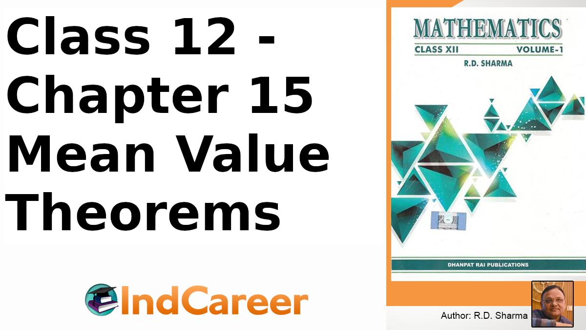
(ii) f (x) = sin 2x on [0, π/2]
Solution:

(iii) f (x) = cos 2x on [-π/4, π/4]
Solution:


sin 2c = 0
⇒ 2c = 0
So,
c = 0 as c ∈ (-π/4, π/4)
∴ Rolle’s Theorem is verified.
(iv) f (x) = ex sin x on [0, π]
Solution:
Given function is f (x) = ex sin x on [0, π]
We know that exponential and sine functions are continuous and differentiable on R. Let’s find the values of the function at an extreme,


(v) f (x) = ex cos x on [-π/2, π/2]
Solution:


(vi) f (x) = cos 2x on [0, π]
Solution:
Given function is f (x) = cos 2x on [0, π]
We know that cosine function is continuous and differentiable on R. Let’s find the values of function at extreme,
⇒ f (0) = cos2(0)
⇒ f (0) = cos(0)
⇒ f (0) = 1
⇒ f (π) = cos2( )
)
⇒ f (π) = cos(2 π)
⇒ f (π) = 1
We have f (0) = f (π), so there exist a c belongs to (0, π) such that f’(c) = 0.
Let’s find the derivative of f(x)

sin 2c = 0
So, 2c = 0 or π
c = 0 or π/2
But,
c = π/2 as c ∈ (0, π)
Hence, Rolle’s Theorem is verified.

Solution:


(viii) f (x) = sin 3x on [0, π]
Solution:
Given function is f (x) = sin3x on [0, π]
We know that sine function is continuous and differentiable on R. Let’s find the values of function at extreme,
⇒ f (0) = sin3(0)
⇒ f (0) = sin0
⇒ f (0) = 0
⇒ f (π) = sin3(π)
⇒ f (π) = sin(3 π)
⇒ f (π) = 0
We have f (0) = f (π), so there exist a c belongs to (0, π) such that f’(c) = 0.
Let’s find the derivative of f(x)


Solution:


(x) f (x) = log (x2 + 2) – log 3 on [-1, 1]
Solution:
Given function is f (x) = log(x2 + 2) – log3 on [– 1, 1]
We know that logarithmic function is continuous and differentiable in its own domain. We check the values of the function at the extreme,
⇒ f (– 1) = log((– 1)2 + 2) – log 3
⇒ f (– 1) = log (1 + 2) – log 3
⇒ f (– 1) = log 3 – log 3
⇒ f ( – 1) = 0
⇒ f (1) = log (12 + 2) – log 3
⇒ f (1) = log (1 + 2) – log 3
⇒ f (1) = log 3 – log 3
⇒ f (1) = 0
We have got f (– 1) = f (1). So, there exists a c such that c ϵ (– 1, 1) such that f’(c) = 0.
Let’s find the derivative of the function f,


(xi) f (x) = sin x + cos x on [0, π/2]
Solution:


(xii) f (x) = 2 sin x + sin 2x on [0, π]
Solution:
Given function is f (x) = 2sinx + sin2x on [0, π]
We know that sine function continuous and differentiable over R.
Let’s check the values of function f at the extremes
⇒ f (0) = 2sin(0) + sin2(0)
⇒ f (0) = 2(0) + 0
⇒ f (0) = 0
⇒ f (π) = 2sin(π) + sin2(π)
⇒ f (π) = 2(0) + 0
⇒ f (π) = 0
We have f (0) = f (π), so there exist a c belongs to (0, π) such that f’(c) = 0.
Let’s find the derivative of function f.

⇒ f’(x) = 2cosx + 2cos2x
⇒ f’(x) = 2cosx + 2(2cos2x – 1)
⇒ f’(x) = 4 cos2x + 2 cos x – 2
We have f’(c) = 0,
⇒ 4cos2c + 2 cos c – 2 = 0
⇒ 2cos2c + cos c – 1 = 0
⇒ 2cos2c + 2 cos c – cos c – 1 = 0
⇒ 2 cos c (cos c + 1) – 1 (cos c + 1) = 0
⇒ (2cos c – 1) (cos c + 1) = 0


Solution:


Solution:


(xv) f (x) = 4sin x on [0, π]
Solution:


(xvi) f (x) = x2 – 5x + 4 on [0, π/6]
Solution:
Given function is f (x) = x2 – 5x + 4 on [1, 4]
Since, given function f is a polynomial it is continuous and differentiable everywhere i.e., on R.
Let us find the values at extremes
⇒ f (1) = 12 – 5(1) + 4
⇒ f (1) = 1 – 5 + 4
⇒ f (1) = 0
⇒ f (4) = 42 – 5(4) + 4
⇒ f (4) = 16 – 20 + 4
⇒ f (4) = 0
We have f (1) = f (4). So, there exists a c ϵ (1, 4) such that f’(c) = 0.
Let’s find the derivative of f(x):

(xvii) f (x) = sin4 x + cos4 x on [0, π/2]
Solution:


(xviii) f (x) = sin x – sin 2x on [0, π]
Solution:
Given function is f (x) = sin x – sin2x on [0, π]
We know that sine function is continuous and differentiable over R.
Now we have to check the values of the function ‘f’ at the extremes.
⇒ f (0) = sin (0)–sin 2(0)
⇒ f (0) = 0 – sin (0)
⇒ f (0) = 0
⇒ f (π) = sin(π) – sin2(π)
⇒ f (π) = 0 – sin(2π)
⇒ f (π) = 0
We have f (0) = f (π). So, there exists a c ϵ (0, π) such that f’(c) = 0.
Now we have to find the derivative of the function ‘f’

4. Using Rolle’s Theorem, find points on the curve y = 16 – x2, x ∈ [-1, 1], where tangent is parallel to x – axis.
Solution:
Given function is y = 16 – x2, x ϵ [– 1, 1]
We know that polynomial function is continuous and differentiable over R.
Let us check the values of ‘y’ at extremes
⇒ y (– 1) = 16 – (– 1)2
⇒ y (– 1) = 16 – 1
⇒ y (– 1) = 15
⇒ y (1) = 16 – (1)2
⇒ y (1) = 16 – 1
⇒ y (1) = 15
We have y (– 1) = y (1). So, there exists a c ϵ (– 1, 1) such that f’(c) = 0.
We know that for a curve g, the value of the slope of the tangent at a point r is given by g’(r).
Now we have to find the derivative of curve y
⇒

⇒ y’ = – 2x
We have y’(c) = 0
⇒ – 2c = 0
⇒ c = 0 ϵ (– 1, 1)
Value of y at x = 1 is
⇒ y = 16 – 02
⇒ y = 16
∴ The point at which the curve y has a tangent parallel to x – axis (since the slope of x – axis is 0) is (0, 16).
Exercise 15.2 Page No: 15.17
1. Verify Lagrange’s mean value theorem for the following functions on the indicated intervals. In each case find a point ‘c’ in the indicated interval as stated by the Lagrange’s mean value theorem:
(i) f (x) = x2 – 1 on [2, 3]
Solution:


(ii) f (x) = x3 – 2x2 – x + 3 on [0, 1]
Solution:
Given f (x) = x3 – 2x2 – x + 3 on [0, 1]
Every polynomial function is continuous everywhere on (−∞, ∞) and differentiable for all arguments. Here, f(x) is a polynomial function. So it is continuous in [0, 1] and differentiable in (0, 1). So both the necessary conditions of Lagrange’s mean value theorem is satisfied.
Therefore, there exist a point c ∈ (0, 1) such that:

f (x) = x3 – 2x2 – x + 3
Differentiating with respect to x
f’(x) = 3x2 – 2(2x) – 1
= 3x2 – 4x – 1
For f’(c), put the value of x=c in f’(x)
f’(c)= 3c2 – 4c – 1
For f (1), put the value of x = 1 in f(x)
f (1)= (1)3 – 2(1)2 – (1) + 3
= 1 – 2 – 1 + 3
= 1
For f (0), put the value of x=0 in f(x)
f (0)= (0)3 – 2(0)2 – (0) + 3
= 0 – 0 – 0 + 3
= 3
∴ f’(c) = f(1) – f(0)
⇒ 3c2 – 4c – 1 = 1 – 3
⇒ 3c2 – 4c = 1 + 1 – 3
⇒ 3c2 – 4c = – 1
⇒ 3c2 – 4c + 1 = 0
⇒ 3c2 – 3c – c + 1 = 0
⇒ 3c(c – 1) – 1(c – 1) = 0
⇒ (3c – 1) (c – 1) = 0

(iii) f (x) = x (x – 1) on [1, 2]
Solution:
Given f (x) = x (x – 1) on [1, 2]
= x2 – x
Every polynomial function is continuous everywhere on (−∞, ∞) and differentiable for all arguments. Here, f(x) is a polynomial function. So it is continuous in [1, 2] and differentiable in (1, 2). So both the necessary conditions of Lagrange’s mean value theorem is satisfied.
Therefore, there exist a point c ∈ (1, 2) such that:

f (x) = x2 – x
Differentiating with respect to x
f’(x) = 2x – 1
For f’(c), put the value of x=c in f’(x):
f’(c)= 2c – 1
For f (2), put the value of x = 2 in f(x)
f (2) = (2)2 – 2
= 4 – 2
= 2
For f (1), put the value of x = 1 in f(x):
f (1)= (1)2 – 1
= 1 – 1
= 0
∴ f’(c) = f(2) – f(1)
⇒ 2c – 1 = 2 – 0
⇒ 2c = 2 + 1
⇒ 2c = 3

(iv) f (x) = x2 – 3x + 2 on [-1, 2]
Solution:
Given f (x) = x2 – 3x + 2 on [– 1, 2]
Every polynomial function is continuous everywhere on (−∞, ∞) and differentiable for all arguments. Here, f(x) is a polynomial function. So it is continuous in [– 1, 2] and differentiable in (– 1, 2). So both the necessary conditions of Lagrange’s mean value theorem is satisfied.
Therefore, there exist a point c ∈ (-1, 2) such that:

f (x) = x2 – 3x + 2
Differentiating with respect to x
f’(x) = 2x – 3
For f’(c), put the value of x = c in f’(x):
f’(c)= 2c – 3
For f (2), put the value of x = 2 in f(x)
f (2) = (2)2 – 3 (2) + 2
= 4 – 6 + 2
= 0
For f (– 1), put the value of x = – 1 in f(x):
f (– 1) = (– 1)2 – 3 (– 1) + 2
= 1 + 3 + 2
= 6

⇒ 2c = 1
⇒ c = ½ ∈ (-1, 2)
Hence, Lagrange’s mean value theorem is verified.
(v) f (x) = 2x2 – 3x + 1 on [1, 3]
Solution:
Given f (x) = 2x2 – 3x + 1 on [1, 3]
Every polynomial function is continuous everywhere on (−∞, ∞) and differentiable for all arguments. Here, f(x) is a polynomial function. So it is continuous in [1, 3] and differentiable in (1, 3). So both the necessary conditions of Lagrange’s mean value theorem is satisfied.
Therefore, there exist a point c ∈ (1, 3) such that:

f (x) = 2x2 – 3x + 1
Differentiating with respect to x
f’(x) = 2(2x) – 3
= 4x – 3
For f’(c), put the value of x = c in f’(x):
f’(c)= 4c – 3
For f (3), put the value of x = 3 in f(x):
f (3) = 2 (3)2 – 3 (3) + 1
= 2 (9) – 9 + 1
= 18 – 8 = 10
For f (1), put the value of x = 1 in f(x):
f (1) = 2 (1)2 – 3 (1) + 1
= 2 (1) – 3 + 1
= 2 – 2 = 0

(vi) f (x) = x2 – 2x + 4 on [1, 5]
Solution:
Given f (x) = x2 – 2x + 4 on [1, 5]
Every polynomial function is continuous everywhere on (−∞, ∞) and differentiable for all arguments. Here, f(x) is a polynomial function. So it is continuous in [1, 5] and differentiable in (1, 5). So both the necessary conditions of Lagrange’s mean value theorem is satisfied.
Therefore, there exist a point c ∈ (1, 5) such that:

f (x) = x2 – 2x + 4
Differentiating with respect to x:
f’(x) = 2x – 2
For f’(c), put the value of x=c in f’(x):
f’(c)= 2c – 2
For f (5), put the value of x=5 in f(x):
f (5)= (5)2 – 2(5) + 4
= 25 – 10 + 4
= 19
For f (1), put the value of x = 1 in f(x)
f (1) = (1)2 – 2 (1) + 4
= 1 – 2 + 4
= 3

(vii) f (x) = 2x – x2 on [0, 1]
Solution:
Given f (x) = 2x – x2 on [0, 1]
Every polynomial function is continuous everywhere on (−∞, ∞) and differentiable for all arguments. Here, f(x) is a polynomial function. So it is continuous in [0, 1] and differentiable in (0, 1). So both the necessary conditions of Lagrange’s mean value theorem is satisfied.
Therefore, there exist a point c ∈ (0, 1) such that:

⇒ f’(c) = f(1) – f(0)
f (x) = 2x – x2
Differentiating with respect to x:
f’(x) = 2 – 2x
For f’(c), put the value of x = c in f’(x):
f’(c)= 2 – 2c
For f (1), put the value of x = 1 in f(x):
f (1)= 2(1) – (1)2
= 2 – 1
= 1
For f (0), put the value of x = 0 in f(x):
f (0) = 2(0) – (0)2
= 0 – 0
= 0
f’(c) = f(1) – f(0)
⇒ 2 – 2c = 1 – 0
⇒ – 2c = 1 – 2
⇒ – 2c = – 1

(viii) f (x) = (x – 1) (x – 2) (x – 3)
Solution:
Given f (x) = (x – 1) (x – 2) (x – 3) on [0, 4]
= (x2 – x – 2x + 2) (x – 3)
= (x2 – 3x + 2) (x – 3)
= x3 – 3x2 + 2x – 3x2 + 9x – 6
= x3 – 6x2 + 11x – 6 on [0, 4]
Every polynomial function is continuous everywhere on (−∞, ∞) and differentiable for all arguments. Here, f(x) is a polynomial function. So it is continuous in [0, 4] and differentiable in (0, 4). So both the necessary conditions of Lagrange’s mean value theorem is satisfied.
Therefore, there exist a point c ∈ (0, 4) such that:

f (x) = x3 – 6x2 + 11x – 6
Differentiating with respect to x:
f’(x) = 3x2 – 6(2x) + 11
= 3x2 – 12x + 11
For f’(c), put the value of x = c in f’(x):
f’(c) = 3c2 – 12c + 11
For f (4), put the value of x = 4 in f(x):
f (4) = (4)3 – 6(4)2 + 11 (4) – 6
= 64 – 96 + 44 – 6
= 6
For f (0), put the value of x = 0 in f(x):
f (0) = (0)3 – 6 (0)2 + 11 (0) – 6
= 0 – 0 + 0 – 6
= – 6

3c2 – 12c + 11 = [6 – (-6)]/ 4
3c2 – 12c + 11 = 12/4
3c2 – 12c + 11 = 3
3c2 – 12c + 8 = 0


Solution:


(x) f (x) = tan-1x on [0, 1]
Solution:
Given f (x) = tan – 1 x on [0, 1]
Tan – 1 x has unique value for all x between 0 and 1.
∴ f (x) is continuous in [0, 1]
f (x) = tan – 1 x
Differentiating with respect to x:

x2 always has value greater than 0.
⇒ 1 + x2 > 0
∴ f (x) is differentiable in (0, 1)
So both the necessary conditions of Lagrange’s mean value theorem is satisfied. Therefore, there exist a point c ∈ (0, 1) such that:


Solution:


(xii) f (x) = x (x + 4)2 on [0, 4]
Solution:
Given f (x) = x (x + 4)2 on [0, 4]
= x [(x)2 + 2 (4) (x) + (4)2]
= x (x2 + 8x + 16)
= x3 + 8x2 + 16x on [0, 4]
Every polynomial function is continuous everywhere on (−∞, ∞) and differentiable for all arguments. Here, f(x) is a polynomial function. So it is continuous in [0, 4] and differentiable in (0, 4). So both the necessary conditions of Lagrange’s mean value theorem is satisfied. Therefore, there exist a point c ∈ (0, 4) such that:

f (x) = x3 + 8x2 + 16x
Differentiating with respect to x:
f’(x) = 3x2 + 8(2x) + 16
= 3x2 + 16x + 16
For f’(c), put the value of x = c in f’(x):
f’(c)= 3c2 + 16c + 16
For f (4), put the value of x = 4 in f(x):
f (4)= (4)3 + 8(4)2 + 16(4)
= 64 + 128 + 64
= 256
For f (0), put the value of x = 0 in f(x):
f (0)= (0)3 + 8(0)2 + 16(0)
= 0 + 0 + 0
= 0


Solution:


(xiv) f (x) = x2 + x – 1 on [0, 4]
Solution:
Given f (x) = x2 + x – 1 on [0, 4]
Every polynomial function is continuous everywhere on (−∞, ∞) and differentiable for all arguments. Here, f(x) is a polynomial function. So it is continuous in [0, 4] and differentiable in (0, 4). So both the necessary conditions of Lagrange’s mean value theorem is satisfied. Therefore, there exist a point c ∈ (0, 4) such that:

f (x) = x2 + x – 1
Differentiating with respect to x:
f’(x) = 2x + 1
For f’(c), put the value of x = c in f’(x):
f’(c) = 2c + 1
For f (4), put the value of x = 4 in f(x):
f (4)= (4)2 + 4 – 1
= 16 + 4 – 1
= 19
For f (0), put the value of x = 0 in f(x):
f (0) = (0)2 + 0 – 1
= 0 + 0 – 1
= – 1


(xv) f (x) = sin x – sin 2x – x on [0, π]
Solution:
Given f (x) = sin x – sin 2x – x on [0, π]
Sin x and cos x functions are continuous everywhere on (−∞, ∞) and differentiable for all arguments. So both the necessary conditions of Lagrange’s mean value theorem is satisfied. Therefore, there exist a point c ∈ (0, π) such that:


(xvi) f (x) = x3 – 5x2 – 3x on [1, 3]
Solution:
Given f (x) = x3 – 5x2 – 3x on [1, 3]
Every polynomial function is continuous everywhere on (−∞, ∞) and differentiable for all arguments. Here, f(x) is a polynomial function. So it is continuous in [1, 3] and differentiable in (1, 3). So both the necessary conditions of Lagrange’s mean value theorem is satisfied.
Therefore, there exist a point c ∈ (1, 3) such that:

f (x) = x3 – 5x2 – 3x
Differentiating with respect to x:
f’(x) = 3x2 – 5(2x) – 3
= 3x2 – 10x – 3
For f’(c), put the value of x=c in f’(x):
f’(c)= 3c2 – 10c – 3
For f (3), put the value of x = 3 in f(x):
f (3)= (3)3 – 5(3)2 – 3(3)
= 27 – 45 – 9
= – 27
For f (1), put the value of x = 1 in f(x):
f (1)= (1)3 – 5 (1)2 – 3 (1)
= 1 – 5 – 3
= – 7

⇒ 3c2 – 10c – 3 = – 10
⇒ 3c2 – 10c – 3 + 10 = 0
⇒ 3c2 – 10c + 7 = 0
⇒ 3c2 – 7c – 3c + 7 = 0
⇒ c (3c – 7) – 1(3c – 7) = 0
⇒ (3c – 7) (c – 1) = 0

2. Discuss the applicability of Lagrange’s mean value theorem for the function f(x) = |x| on [– 1, 1].
Solution:


3. Show that the Lagrange’s mean value theorem is not applicable to the function f(x) = 1/x on [–1, 1].
Solution:
Given

Here, x ≠ 0
⇒ f (x) exists for all values of x except 0
⇒ f (x) is discontinuous at x=0
∴ f (x) is not continuous in [– 1, 1]
Hence the Lagrange’s mean value theorem is not applicable to the function f (x) = 1/x on [-1, 1]
4. Verify the hypothesis and conclusion of Lagrange’s mean value theorem for the function

Solution:
Given


5. Find a point on the parabola y = (x – 4)2, where the tangent is parallel to the chord joining (4, 0) and (5, 1).
Solution:
Given f(x) = (x – 4)2 on [4, 5]
This interval [a, b] is obtained by x – coordinates of the points of the chord.
Every polynomial function is continuous everywhere on (−∞, ∞) and differentiable for all arguments. Here, f(x) is a polynomial function. So it is continuous in [4, 5] and differentiable in (4, 5). So both the necessary conditions of Lagrange’s mean value theorem is satisfied.
Therefore, there exist a point c ∈ (4, 5) such that:

⇒ f’(x) = 2 (x – 4) (1)
⇒ f’(x) = 2 (x – 4)
For f’(c), put the value of x=c in f’(x):
f’(c) = 2 (c – 4)
For f (5), put the value of x=5 in f(x):
f (5) = (5 – 4)2
= (1)2
= 1
For f (4), put the value of x=4 in f(x):
f (4) = (4 – 4)2
= (0)2
= 0
f’(c) = f(5) – f(4)
⇒ 2(c – 4) = 1 – 0
⇒ 2c – 8 = 1
⇒ 2c = 1 + 8

We know that, the value of c obtained in Lagrange’s Mean value Theorem is nothing but the value of x – coordinate of the point of the contact of the tangent to the curve which is parallel to the chord joining the points (4, 0) and (5, 1).
Now, put this value of x in f(x) to obtain y:
y = (x – 4)2

RD Sharma Solutions for Class 12 Maths Chapter 15: Download PDF
RD Sharma Solutions for Class 12 Maths Chapter 15–Mean Value Theorems
Download PDF: RD Sharma Solutions for Class 12 Maths Chapter 15–Mean Value Theorems PDF
Chapterwise RD Sharma Solutions for Class 12 Maths :
- Chapter 1–Relation
- Chapter 2–Functions
- Chapter 3–Binary Operations
- Chapter 4–Inverse Trigonometric Functions
- Chapter 5–Algebra of Matrices
- Chapter 6–Determinants
- Chapter 7–Adjoint and Inverse of a Matrix
- Chapter 8–Solution of Simultaneous Linear Equations
- Chapter 9–Continuity
- Chapter 10–Differentiability
- Chapter 11–Differentiation
- Chapter 12–Higher Order Derivatives
- Chapter 13–Derivatives as a Rate Measurer
- Chapter 14–Differentials, Errors and Approximations
- Chapter 15–Mean Value Theorems
- Chapter 16–Tangents and Normals
- Chapter 17–Increasing and Decreasing Functions
- Chapter 18–Maxima and Minima
- Chapter 19–Indefinite Integrals
About RD Sharma
RD Sharma isn’t the kind of author you’d bump into at lit fests. But his bestselling books have helped many CBSE students lose their dread of maths. Sunday Times profiles the tutor turned internet star
He dreams of algorithms that would give most people nightmares. And, spends every waking hour thinking of ways to explain concepts like ‘series solution of linear differential equations’. Meet Dr Ravi Dutt Sharma — mathematics teacher and author of 25 reference books — whose name evokes as much awe as the subject he teaches. And though students have used his thick tomes for the last 31 years to ace the dreaded maths exam, it’s only recently that a spoof video turned the tutor into a YouTube star.
R D Sharma had a good laugh but said he shared little with his on-screen persona except for the love for maths. “I like to spend all my time thinking and writing about maths problems. I find it relaxing,” he says. When he is not writing books explaining mathematical concepts for classes 6 to 12 and engineering students, Sharma is busy dispensing his duty as vice-principal and head of department of science and humanities at Delhi government’s Guru Nanak Dev Institute of Technology.